Dear Salonnières,
thanks for attending compu-salon episode 10, high-performance Python. This was the last of my... performances for this year; we will now switch to a show-and-tell format where you can come and talk about your favorite topic in computing. So every week I will ask for a volunteer, and we shall only meet if there is one.
Anybody for this Friday the 13th? (Jason won't be there.) You know we're so nice and we have fun together... so volunteer.
Now here's a summary of last week's discussion.
Michele
Compu-salon ep. 10 in summary
We again worked with our favorite numerical example, the Mandelbrot set, and did it in six different ways, using a variety of tools to increase performance. Let's go through them again.
[By the way, Ian Ozsvald has a similar tutorial, with more technical detail than perhaps you may want. I was inspired by his code in my numexpr and pyCUDA examples.]
Regular interpreted Python
CPython is Guido van Rossum's reference interpreter for the Python programming language. It's the standard and it's very robust, but of course it can't be optimized for everything. Here's our pure-Python code for the Mandelbrot set, using native complex numbers, and nested lists to hold arrays:
from __future__ import division     # make integer division return a float

x0, x1 = -2, 1                      # computational domain
y0, y1 = -1, 1

def mandel_python(n=400,maxi=512):
    """Compute an n x n Mandelbrot matrix with maxi maximum iterations."""

    dx, dy = (x1-x0)/(n-1), (y1-y0)/(n-1)

    # create array of complex coordinates
    xs = [x0 + i*dx for i in range(n)]
    ys = [y0 + i*dy for i in range(n)]

    result = []                     # use a list to collect matrix rows...
    for y in ys:
        row = []                    # ...and multiple row lists
        for x in xs:                # to collect row elements
            z, c = 0, x + 1j*y      # 1j = math.sqrt(-1)

            escape = maxi           # default result
            for i in range(1,maxi): # Mandelbrot iteration
                z = z*z + c

                if abs(z) > 2:
                    escape = i
                    break

            row.append(escape)
        result.append(row)

    return result
We visualize the result with matplotlib:
import matplotlib.pyplot as P

P.figure()
P.imshow(N.array(mandel_python()),origin='lower',extent=(x0,x1,y0,y1))
P.show()
On my laptop, the Python version takes 5.88 seconds with the default n and maxi parameters, and produces this figure:
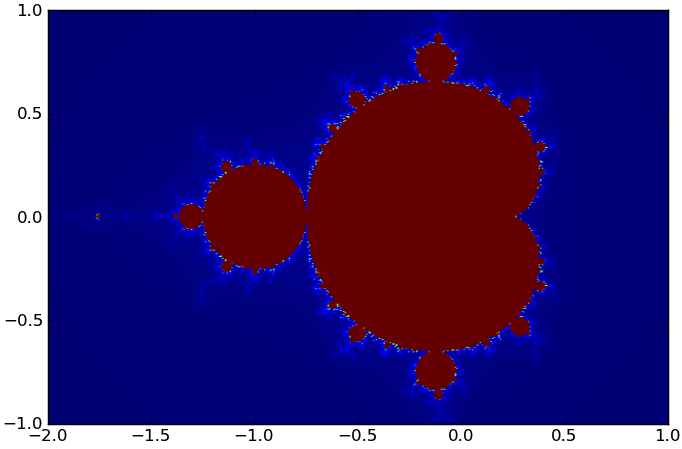
The Mandelbrot set produced by our code
PyPy
There are other implementations of the Python interpreter, which emphasize different case uses, and may have limitations or extensions with respect to the standard language (for instance, interoperability with Java or C#, concurrence)
PyPy is a very interesting variant that bills itself, paradoxically, as "a Python implementation in Python", but it comes with a just-in-time compiler that can provide impressive performance compared to CPython, thanks to a lot of very advanced computer science. (When I look at their development site, half of the time I don't know what they are talking about!)
Right now, however, there is still a drawback. Because of optimization, PyPy does not have access to the broad ecosystem of C- or Fortran-based extensions that work with numpy arrays and leverage legacy code. (It is possible, but not easy, to write extension modules expressly for PyPy.)
Still, if you have only Python code, give it a try. Our example above, using pypy instead of python with the very same mandel_python() code, runs in 0.56 seconds. That is impressive!
numpy
Next is our old friend numpy, which provides general array objects for Python. The array operations are implemented internally in C, so we expect them to be efficient. Writing numpy code however can be wasteful because compound mathematical expressions lead to the creation of lots of temporary objects.
Take for instance the expression a[:] = b[:] * (c[:] + d[:]), where all the operands are numpy arrays. To evaluate it, numpy would create a temporary object to hold c + d, and fill it with the sum; another temporary object to hold the result of the product with b; and finally copy the values into a. Moreover, if the logic of our program includes branches (different things that happen based on the value of some variables), the code can get a little awkward. See our Mandelbrot code:
import numpy as N

def mandel_numpy(n=400,maxi=512):
    """Compute an n x n Mandelbrot matrix with maxi maximum iterations."""

    # get 2-d arrays for x and y, using numpy's convenience function
    xs, ys = N.meshgrid(N.linspace(x0,x1,n), N.linspace(y0,y1,n))

    z = N.zeros((n,n),'complex128')     # a matrix of complex zeros
    c = xs + 1j*ys

    escape = N.empty((n,n),'int32')
    escape[:,:] = maxi                  # default result

    for i in xrange(1,maxi):
        mask = (escape == maxi)         # find out which points have not escaped
                                        # yet (results in a boolean array)

        z[mask] = z[mask]**2 + c[mask]  # run the Mandelbrot iteration only
                                        # on those points, using boolean indexing

        escape[mask & (N.abs(z) > 2)] = i   # if are just escaping now,
                                            # set the result to this iteration

    return escape
Because of these inefficiencies, this version does not run especially fast: 5.6 seconds on my laptop. I should say however that numpy is almost always a good place to start with numerical calculations, since optimizations can be tuned manually in tight spots (as we'll see in the rest of these notes); furthermore, if you have matrix calculations, numpy can access highly-optimized BLAS and LAPACK implementations.
numexpr
numexpr is effectively a just-in-time compiler for numpy, which takes matrix expression (given, somewhat awkwardly, as strings) and creates an efficient representation for the element-wise expressions that generate the final matrix result. Furthermore, numexpr arranges for those expressions to be evaluated in efficients chunks, using multiple threads (which you can set with numexpr.set_num_threads()). Modifying mandel_numpy for numexpr is very easy: it involves inserting calls to numexpr's main function, evaluate, at three numpy-heavy locations.
import numexpr as NE

def mandel_numexpr(n=400,maxi=512):
    """Compute an n x n Mandelbrot matrix with maxi maximum iterations."""

    xs, ys = N.meshgrid(N.linspace(x0,x1,n), N.linspace(y0,y1,n))

    z = N.zeros((n,n),'complex128')
    c = xs + 1j*ys

    escape = N.empty((n,n),'int32')
    escape[:,:] = maxi

    for i in xrange(1,maxi):
        # we're just wrapping the numpy expression with `evaluate`
        mask = NE.evaluate('escape == maxi')

        # boolean indexing is not too numexpr-friendly, so instead we use
        # the numpy function `where(cond,then,else)` and set z to 0
        # at already-escaped points, to avoid overflows
        z = NE.evaluate('where(mask,z**2+c,0)')

        # again where; taking the real part of abs is necessary here
        # because in numexpr abs(complex) is complex with 0 imaginary part
        escape = NE.evaluate('where(mask & (abs(z).real > 2),i,escape)')

    return escape
Using a single thread, the code runs in 2.06 seconds. Not bad for such an easy optimization, but still slower than PyPy.
Cython
Cython is a true compiler for Python. It generates C code from Python source, which by itself is not a big optimization, because the compiled code needs to use the Python interpreter (technically, the Python C API) to handle objects. The real gains come when you start annotating the Python code to specify the types of objects, so that types are determined at compile time rather than at runtime, as it would happen normally with Python. Operations objects of known types can then stay in pure C, which makes them very fast.
The natural optimization style in Cython is to work with numpy arrays, but operate on them element by element. For Mandelbrot, this means using the logic of mandel_python():
# --- file cythonmandel.pyx ---

import numpy as N
cimport numpy as N      # this Cython-side numpy import is needed
                        # to declare the types and dimensions of arrays

x0, x1 = -2.0, 1.0
y0, y1 = -1.0, 1.0

def mandel_cython(int n=400,int maxi=512):
    # declare the type and dimension of numpy arrays
    # (and create them in the same line, C-style)
    cdef N.ndarray[double,ndim=1] xs = N.linspace(x0,x1,n)
    cdef N.ndarray[double,ndim=1] ys = N.linspace(y0,y1,n)

    cdef N.ndarray[int,ndim=2] escape = N.empty((n,n),'int32')

    # declare integer counters
    cdef int i,j,it,esc

    # declare complex variables
    cdef double complex z,c

    for i in range(n):
        for j in range(n):
            z = 0 + 0j
            c = xs[i] + 1j * ys[j]

            esc = maxi
            for it in range(maxi):
                z = z*z + c

                # let's allow ourselves one hand-tuned optimization,
                # which avoids the sqrt implicit in abs
                if z.real*z.real + z.imag*z.imag > 4:
                    esc = it
                    break

            escape[j,i] = esc

    return escape
This file is compiled to cythonmandel.c with cython cythonmandel.pyx; the resulting C file is then compiled to a C extension with
$ PYTHON_INCLUDE=`python -c "import distutils; print distutils.sysconfig.get_python_inc()"`
$ NUMPY_INCLUDE=`python -c "import numpy; print numpy.get_include()"`

$ gcc -std=c99 -O3 -bundle -undefined dynamic_lookup \
     -I$PYTHON_INCLUDE -I$NUMPY_INCLUDE cythonmandel.c -o cythonmandel.so
This is on OS X; on Linux, -shared will do instead of -bundle -undefined dynamic_lookup. The extension is loaded in Python with import cythonmandel, and the function can be used as cythonmandel.mandel_cython().
Doing all this work (it's not so bad, really) gets us a crazy-fast runtime of 0.11 seconds. Definitely worth the work! Cython can also parallelize loops over threads, although in this case it does not help too much.
CUDA
For the grand finale, we'll gain access to the massively parallel processor embedded in all modern computers: the GPU. This is a fine example of scientific computation reaping the benefits of a consumer market—specifically, high-end graphical performance for videogames.
Programming GPUs for general purposes is getting easier, but it is still fraught with pitfalls and difficulty. That is because GPUs were originally designed to perform a very specialized task: painting textures on three-dimensional surfaces, illuminating them, etc. Let me assure you, you don't want to get down to the level of recasting your scientific computation as a 3-D shader.
Fortunately, there are now abstraction libraries that hide the low-level operation of GPUs, and even let us work with numpy objects (with the PyCUDA library). There is one important thing to remember though: the GPU memory is distinct from CPU memory, and data needs to be transferred to and fro manually. With the numpy-array abstraction, this is achieved by creating GPU arrays.
So here's the Mandelbrot code:
import pycuda.autoinit
import pycuda.gpuarray as gpuarray

def mandel_cuda(n=400,maxi=512):
    xs, ys = N.meshgrid(N.linspace(x0,x1,n), N.linspace(y0,y1,n))
    c = xs + 1j*ys

    # the GPU on my laptop does not support double precision floating point,
    # so we define c and z as single-precision complex arrays
    c = c.astype(N.complex64)
    z = N.zeros(c.shape,N.complex64)

    # transfer arrays to the GPU
    zg = gpuarray.to_gpu(z)
    cg = gpuarray.to_gpu(c)

    # create a result array
    outputg = gpuarray.to_gpu(maxi*N.ones(zg.shape,N.int32))

    # because the GPU computing elements can only see the GPU arrays,
    # and not the Python variables on the CPU, if we need constants
    # (here 0 and 2), temporary variables, or counters, we need to
    # create them as GPU arrays
    twog  = gpuarray.to_gpu(2.0*N.ones(zg.shape,N.float32))
    zerog = gpuarray.to_gpu(N.zeros(zg.shape,N.complex64))
    comp = gpuarray.to_gpu(N.zeros(zg.shape,N.bool))
    iterg = gpuarray.to_gpu(N.ones(zg.shape,N.int32))

    for iter in range(1,maxi):
        zg = zg*zg + cg

        # again abs(z) is complex... that's life
        comp = abs(zg).real > twog

        # `if_positive` works like numpy's `where`
        zg = gpuarray.if_positive(comp,zerog,zg)
        cg = gpuarray.if_positive(comp,zerog,cg)

        outputg = gpuarray.if_positive(comp,iterg,outputg)

        # increment a GPU array to track the CPU variable iter
        iterg = iterg + 1

    # transfer back the result
    return outputg.get()
See below for the considerable amount of configuration needed to get this running. It's a miracle that it works, actually... Under the hood Python is calling the NVIDIA CUDA compiler to generate PGU code. So the code gets faster if it's run twice (it reuses the compiled kernel the second time it runs).
In exchange for this annoyance, we get a warmed-up runtime of 2.07 seconds. My laptop's GPU is weak! Plus, there is still overhead from the matrix operations. We can use a lower-level (but still bearable) interface to the GPU by programming the GPU elements explicitly using the C-like CUDA language:
import pycuda.elementwise as elementwise

def python_cudaelement(n=400,maxi=512):
    xs, ys = N.meshgrid(N.linspace(x0,x1,n), N.linspace(y0,y1,n))
    c = xs + 1j*ys

    c = c.astype(N.complex64)
    z = N.zeros(c.shape,N.complex64)

    zg = gpuarray.to_gpu(z)
    cg = gpuarray.to_gpu(c)

    outputg = gpuarray.to_gpu(maxi*N.ones(zg.shape,N.int32))

    # we compile C-like code for the operations that happen on each GPU element;
    # since we can include constants and counters in the code, we don't need
    # to upload them as GPU arrays; note that we don't need to loop explicitly
    # over the array rows and columns, and that we list arguments at the beginning
    mandel_gpu = elementwise.ElementwiseKernel(
        "pycuda::complex<float> *z, pycuda::complex<float> *c, int *output, int maxi",
        """for (int n=1; n<maxi; n++) {
            z[i] = z[i]*z[i] + c[i];

            if(abs(z[i]) > 2.0f) {
                output[i] = n;

                z[i] = pycuda::complex<float>();
                c[i] = pycuda::complex<float>();
            };
        };""",
        "mandel",                                   # name of the kernel
        preamble="#include <pycuda-complex.hpp>",   # needed for complex numbers
        keep=True                                   # cache kernel
    )

    # call the kernel with our arrays
    mandel_gpu(zg,cg,outputg,maxi)

    return outputg.get()
Very dense code, but still readable. With this logic, the runtime gets to 0.25 seconds. Still not as good as Cython, but better than anything else. A sufficiently powerful GPU would probably beat the Cython code, which runs on the CPU.
Now for the CUDA installation: this is what worked for me on OS X, loosely following Alex Wiltschko. After downloading and installing everything from CUDA:
# set environment variables to point to CUDA (needed also at runtime)
$ export PATH=/usr/local/cuda/bin:$PATH
$ export CUDA_ROOT=/usr/local/cuda

# get and configure pyCUDA
$ git clone http://git.tiker.net/trees/pycuda.git
$ git submodule init
$ git submodule update
$ cd pycuda
$ python configure.py

# tweak siteconf.py, removing all references to lib64, and setting
# CXXFLAGS = ['-arch', 'x86_64','-mmacosx-version-min=10.6', '-I' + numpy.get_include()]
# LDFLAGS  = ['-arch', 'x86_64', '-mmacosx-version-min=10.6']

# install pyCUDA
$ make
$ make install
In summary
Whew... here are the final results. You'll notice that in this ugly Excel plot I violated my own precepts, and used a legend. Sorry about that—I promise I'll make it decent. On the x axis, the number of elements in the array (160,000 in the standard case); on the y axis, the warmed-up runtime in seconds. The numexpr numbers are given for 1, 2, and 4 threads; the Cython numbers are given also for parallelized-thread operation, presumably with 4 threads (the maximum number of virtual cores available on my laptop).
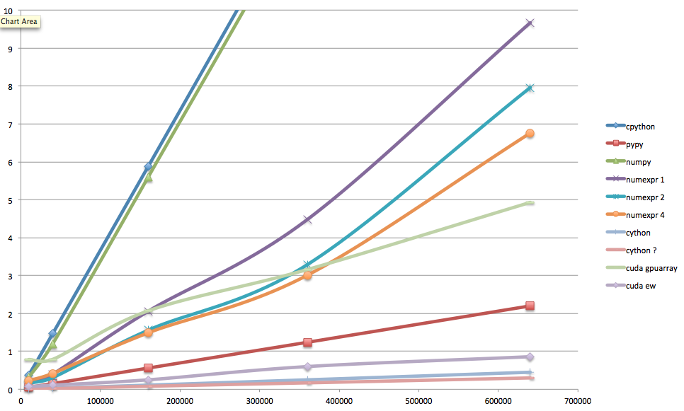
Runtimes for Mandelbrot set, several implementations
What's the takeaway? If you can work in pure Python, try PyPy. Otherwise start with numpy arrays, and optimize with Cython, or with numexpr if you're lazy. If you have access to powerful GPUs with lots of memory, by all means try PyCUDA (or PyOpenCL for ATI GPUs), even if it's still painful and not too elegant.
And this is really all, folks!